MUNI BOND PRICINGFIXED-INCOME ANALYTICS for Municipal Bond issuers
Explanation of Workflow and Calculations
The Calculations of the Municipal Bond Pricing App
Introduction
The calculations that are made by this municipal bond pricing app can be most easily understood as four connected steps. The first step sets the spot-rate curve for both taxable and tax-exempt bonds, with the former referred to as US Treasury spot rates and the latter adjusting these rates to be applicable to municipal bonds. Step two values a non-callable, taxable bond as a risk-free Treasury security using the Treasury spot-rate curve. The third step uses the converted-to-tax-exempt rates to value a non-callable municipal bond. The final step adds the effects of a call feature to value a case where a municipal issuer has an option to pay-off the bond prior to the stated maturity date.
All four steps are explained with example calculations for a 20-year bond that has a 5% coupon with semi-annual payments. A 5% coupon is used because it is common among long-term municipal bonds, while a 20-year maturity makes the effect of a call provision—such as a first call after 10 years—especially clear.
Use NEXT to continue and see how the app was used to estimate a price valuation for this bond.
The Initial Spot Rates and Municipal Bond Rates
Treasury spot rates are a useful starting point (i.e, the first step) because they are widely observed across maturities and are supported by a large, actively-traded market. These rates can be derived from Treasury security prices through bootstrapping or curve fitting procedures (outside the app). A pre-created set of historical, bootstapped Treasury spot rates is provided. The app can also use common Treasury spot-rate curve shapes and facilitate adjustments to such shapes to represent current or expected market conditions.
The initial spot-rate curve serves as an objective benchmark for constructing a tax-free municipal spot-rate curve, which are most easily derived from Treasury rates by applying a tax-shielding adjustment. The resulting municipal curve ultimately warrants the closest attention because these rates directly determine the value of the municipal bond.
Most important, the value of the call option depends on the assumptions and calculations that construct the municipal rate curve. These assumptions and calculations are discussed in detail in the explanation of the final step.
Setting Treasury Rates
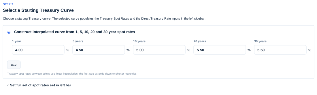
The Treasury spot-rate curve was created by entering rates at five maturities and letting the app interpolate the full curve. The inputs are 4.00% at 1 year, 4.50% at 5 years, 5.00% at 10 years, and 5.50% at both 20 and 30 years. Rates below one year use 4.00%; rates between the entered maturities use linear interpolation.
Each point on the full, interpolated curve then represents the annualized non-tax-exempt return required by investors for a 'spot' payment made 'x' years in the future.
The screenshot above shows the simplest way to set a few Treasury spot rates. There are options using a left bar of inputs (see 'Controls') or the Rate Chart to modify all rates.
Setting an Implied Tax Rate to Derive Municipal Rates
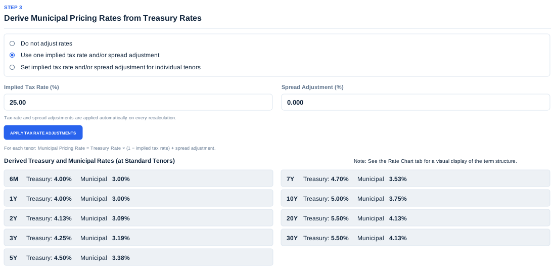
The screenshot below shows a workflow step that creates the municipal bond discount rates from Treasury rates by computing the effect of an assumed federal tax rate of 25% (labelled the implied tax rate). This single value translates the entire Treasury rate curve into values that represent the lower annualized return required by investors for a tax-exempt payment made 'x' years in the future.
In this case, the municipal bond rates are computed from the Treasury rates using this formula:
The Apply Tax Rate Adjustments button then creates a tax-exempt curve that starts at 3.00% at the 6-month mark, rises to 3.75% at 10 years, and reaches 4.125% (displayed as 4.13%) at both 20 and 30 years. Every municipal spot rate is 75% of the corresponding Treasury rate because the implied tax rate is 25% and the spread adjustment is zero.
This step in the workflow provides an option to set implied tax rate and/or spread adjustment for individual tenors or maturities. You can also set the implied tax rate to 0% to value a bond without tax-exempt status.
Display of Treasury and Municipal Bond Rates
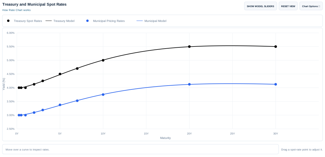
Below is a graphical view of the two sets of rates for the calculations in this example. The higher curve shows taxable Treasury rates and the lower curve shows the corresponding tax-free municipal bond rates.
The black Treasury dots rise from 4.00% to 5.50%, while the blue municipal dots rise from 3.00% to 4.125%. The smooth model lines are NSS fits to the dots; fitting does not replace the spot rates used for pricing.
Using Spot Rates to Value a No-Call Taxable Bond
With the bond terms (coupon rate, maturity date) and discount rates (Treasury and municipal spot rates) set, the price for both a taxable (Treasury) and tax-exempt (municipal) bond without a call option can be calculated.
The Treasury spot rate curve is used in a straightforward manner to compute the present value of taxable payments. In these calculations, the Treasury spot rates (often referred to as risk-free, zero-coupon discount rates) turn promised future payments into a present value price:
In particular, for each $100 of principal, a 5% coupon bond pays $2.50 every six months and the bond’s current value is derived by discounting each future coupon payment to the present using a spot rate that is associated with each payment date. The six-month coupon uses the six-month spot rate, the one-year coupon uses the one-year spot rate, and so forth through the full life of the bond that ends with a principal payment of $100. In this example, the 20-year bond has 40 distinct payments (39 pay $2.50, the final payment pays back the principal as well, or $102.50). In essence, the valuation requires discount factors for each of the 40 semi-annual payment dates.
Using 40 distinct spot rates in the curve, the full sum from the formula is $96.31 (per $100 in par), which is the present value of the bond’s future payments using the given discount rates. The yield-to-maturity or YTM at this price is 5.30%, which can be derived as the implied single interest rate for the formula that produces the same $96.31 per $100 in par price (i.e. the equivalent flat curve).
For the example’s entered issue and settlement date of November 7, 2026, and maturity date of November 7, 2046, the app’s QuantLib calculation gives a clean Treasury bond price of 96.26 and YTM of 5.31%. The value differs slightly from the simplified formula that gives 96.31 as the price because QuantLib uses exact calendar dates and a different day-count convention.
Because every coupon and the principal payment is discounted using a specific spot rate curve , any change in the curve’s level or shape can change the calculated value (irrespective of whether the formula above or the QUANTLIB library is used). The app has many design features that can demonstrate and quantify the sensitivity of both tax-able and tax-free bonds to changes in a spot rate curve. In this example, we hold to using a single taxable curve that serves as a calculation benchmark.
Using Tax-Exempt Rates for Municipal Bonds
For the next step, the tax-adjusted municipal bond rates are applied in the exact same manner. The results produce a higher valuation of 113.75 for the non-callable municipal bond, compared with 96.26 for the taxable Treasury case. Its municipal YTM is 4.00%.
In this example, the municipal bond spot rates were constructed to only reflect the federal tax exemption on coupon payments from municipal issuers. These rates can also be adjusted to reflect the credit status of the issuer and liquidity issues that relate to supply and demand in the municipal-market. In other words, the tax-adjusted Treasury curve can be seen as a starting point for valuing a municipal bond and may not fully reflect rates that appropriately discount the promised payments from all issuers.
Suppose the issuer can redeem the bond for $100 after 10 years at their discretion, as opposed to paying the 5% coupon payments for another 10 years and redeeming at the stated 20-year mark. This ‘call option’ has value for the issuer because it can end the remaining 5% payments when refinancing becomes economical – which will primarily depend on whether refunding rates are above or below 5% at the 10-year mark. In essence, the call option lowers the expected cost of financing from the issuer’s perspective.
The effective cost of committing to the bond’s terms from the issuer’s perspective is computed as:
Expected present value cost of payments =

  Present value of bond payments prior to first call date

  + Probability of call at first call date
      × 100 × (1 + coupon rate/2) × call date discount factor

  + Sum of probability and discount factor weighted payments
      of calls after the first call opportunity

  + Probability of no call
      × 100 × (1 + coupon rate/2) × maturity date discount factor
Each of the probability-based terms reflects the issuer's flexibility to refinance when doing so is financially advantageous. They are derived by modelling future interest rates as a random (stochastic) process with a selected degree of reversion to 'normal'. The app simply recognizes that a 'call' gives the issuer the right, but not the obligation, to redeem the bond and end the payments.
The call decision is largely driven by the bond's coupon rate in relation to the market interest rate, with calls made when the market rate is below the coupon rate (on or after the allowed call date). The app assumes the issuer makes the smart decision by comparing the value of leaving the remaining obligations outstanding with the cost of redeeming or refinancing the bond.
In many cases, the third term is close to zero because the value of calling the bond after the first opportunity, and not at the first opportunity, is low. In essence, a model of potential future interest rates would more often lead to either calling at the first date or never making a call (represented by the last term). In fact, with a 5% coupon rate and starting market rates in the 3.00% to 4.13% range the probability of call at first call date is much higher than any other case.
The formula above simply computes the bond’s value or price as the expected present value of the payments to investors. Another way to look at the call option for the bond is:
Call-option value for issuer =
  Present value of full set of bond payments (no-call case)
  − Callable bond value
Here, the no-call case simply sets the probability of not making a call at any date at 1 (thus the other probabilities are set at zero). It assumes the issuer must make every payment, with a value based on a set discount rate curve that applies through the stated maturity date. Therefore, the call value is based on not needing to fully commit to the full set of payments (i.e., hold an option).
The app recognizes that the call option adds value to the issuer and it correspondingly lowers its value to investors. Note that the option’s perceived cost to any investor may be higher or lower than the perceived value to the issuer (mainly due to risk considerations, market factors, and a higher or lower tax rate for the investor).
Valuation With Call Options
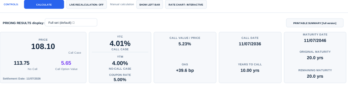
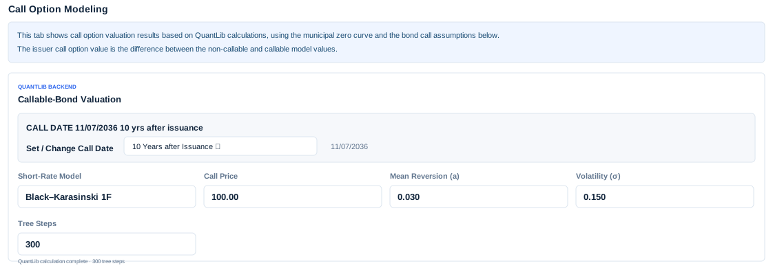
The screenshot below shows the results from assuming a call option at year 10.
The callable bond’s YTC is 4.01%; the no-call municipal YTM is 4.00%. The call value is 5.23% of the callable price.
The value of the bond with a call at 10 years is calculated to be 108.10 and was determined using the same municipal spot rates coupled with interest-rate scenarios built from the Black–Karasinski model with the parameter settings below. Thus, the value of the call is 5.65 (113.748 − 108.099).